Linear Regression #2: Model Specification

Frisch-Waugh Theorem


Assume that we have a regression model with \(\small{ k }\) different variables. In some cases, we might not be interested in all \(\small{ k }\) variables, but in a subset only.
\[y=X\beta+Z\gamma+\varepsilon\]

The theorem uses a projection matrix \(\small{ P=Z^\prime\left(Z^\prime Z\right)^{-1}Z^\prime }\) so that \(\small{ Q=\left(I-P\right)}\). Now, \(\small{ Q }\) is the orthogonal projection onto the column space of \(\small{ Z }\) and therefore eliminates the influence of \(\small{ Z }\).

\[y=X\beta+Z\gamma+\varepsilon \\ \Leftrightarrow\ X^\prime Qy =X^\prime QX\beta+X^\prime QZ\gamma \\ \Leftrightarrow\ X^\prime Qy =\ X^\prime QX\beta \\ \Leftrightarrow\hat{\beta} =\left(X^\prime Q\ X\right)^{-1}\ X^\prime Qy\]

After this transformation, we have our model \(\small{ Qy=QX\beta+Q\varepsilon }\) with the variance \(\small{ \mathbb{V}\left(\hat{\beta}\right)=\sigma^2\left(X^\prime Q\ X\right)^{-1} }\) .
The vectors of the OLS residuals \(\small{ \varepsilon_0=y-(X\hat{\beta}+Z\hat{\gamma}) }\) and \(\small{ \varepsilon_{FW}=Qy-QX\hat{\beta} }\) coincide.

By eliminating \(\small{ Z }\) with Frisch-Waugh, we still capture the effect of \(\small{ Z }\) but without including the additional variables in our model.

Model Misspecification

We call a model misspecified if we discover over- or underspecification. Let’s have a quick look at the difference:

OverspecificationUnderspecification
True Model:
\[y=X\beta+\varepsilon\]
Estimated Model:
\[y=X\beta+Z\omega+\varepsilon\]
Problem:
Overspecification is not a big problem, but the estimation will lose some efficiency.
True Model:
\[y=X\beta+Z\omega+\varepsilon\]
Estimated Model:
\[y=X\beta+\varepsilon\]
Problem:
Underspecification is a severe problem, since our estimated coefficients are incorrect.

The F-test provides a test statistic to identify model misspecification. Let there be two different regression models \(\small{ m0_{N\times K}:\ y=X\beta+\varepsilon }\) and \(\small{ m1_{N\times L}:\ y=X\beta+Z\omega+\varepsilon }\). We assume that \(\small{ m1 }\) is the true model and formulate the hypotheses
\[H_0:\ \omega=0\] or \[H_1:\ \omega\neq0\]

We now calculate the F-statistic, with \(\small{ N-K-L }\) degrees of freedom, where \(\small{ N }\) is the number of rows, and \(\small{ K+L }\) denote the number of columns.
\[F\left(m\right)=\frac{(RSS\left(m0\right)-RSS\left(m1\right))/L}{RSS(m1)/(N-K-L)\ \ }\]

The null hypothesis \(\small{ H0 }\) is rejected at level of significance \(\small{ \alpha }\) , if \(\small{ F\left(m\right)>F_{L,\ \ \ \left[N-K-L\right]}^{1-\alpha} }\) holds.

Bias: Correlation and Underspecification

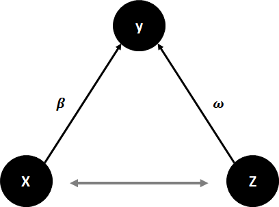
Let’s assume that two regressors \(\small{ \beta_1 }\) and \(\small{ \omega_0 }\) are positively correlated in our model
\[y_i=\beta_0+\beta_1x_i+\omega_0z_i+\varepsilon_i\]
If we now build our regression model without \(\small{ \omega_0 }\) , then \(\small{ {\hat{\beta}}_1 }\) will measure the effect of \(\small{ \omega_0 }\) on \(\small{ y_i }\) and will not be unbiased.

\[Bias\left({\hat{\beta}}_1\right)=\mathbb{E}\left[{\hat{\beta}}_1\right]-\beta_1=\frac{corr(x,z)}{Var(x)}\omega_0\]
If both regressors are positively correlated (and \(\small{ \omega_0>0 }\) ), we expect a positive bias.


Data Science #3: Predictive Modelling

Prediction Models are built on data of the past. A common application is observing a customer’s attributes and behaviour in order to predict whether he will return a purchased item or keep it. Before a model can make such a prediction, it needs to learn from past data that include the outcome label (target variable). After that training process, the model is able to make predictions based on new unlabelled data (=target variable is missing).

Predicitive Analytics: A prediction model is trained with the training data and tested with the testing data.

Predictive Algorithms

1. Regression Models

Linear or non-linear regression algorithms make predictions/forecasts by calculating a model with a continuous dependent target variable.
Typical business cases are sales predictions or financial forecasts.

2. Classification Models

Classification algorithms classify objects into known groups. (Remember: Groups were unknown in cluster analysis). For instance, a dichotomous target variable might be the risk of credit default (1=default, 0=repayment). At the point of loan application, the outcome is not yet known. However, classification models can make a prediction based on the characteristics/attributes of the applicant (object).

Decision Trees

A decision tree is a set of splitting rules that predicts discrete (classification) or continuous (regression) outcomes. It can be visualised as directed tree-like graph starting from a root node, including various splitter nodes and ending with the possible outcomes (leaves).

I want to show you two simple examples of decision trees. First, a classification decision tree that classifies the passengers of the Titanic into two groups: survivors and fatalities.

The second type of decision trees describes a regression model. For instance, take a look at the average income of a person based on different attributes.

Building a Decision Tree

When creating a decision tree, it is our ambition to increase the impurity of the data. That is looking for “good splits” that reduce the impurity and avoiding splits that only fit for few data points.
To measure impurity \(\small{ I\left(N\right) }\) of some node \(\small{ N }\), there are several common choices to take. Two often used impurity criteria are the Entropy \(\small{ I_E\left(N\right) }\) and the Gini Index \(\small{ I_G\left(N\right) }\).

Entropy:

\[I_E\left(N\right)=-\sum_{j=1}^{c}{p_j\log_2{(p_j)}}\]
Gini Index:

\[I_G\left(N\right)=1-\sum_{j=1}^{c}p_j^2\]

\(\small{ p_j=p(y_j|N) }\) denotes the proportion of data points that belongs to class \(\small{ c }\) for node \(\small{ N }\) . The Gini Index can reach a maximum of \(\small{ max{\ I}G\left(N\right)=0.5 }\) and with Entropy \(\small{ max{\ I}_E\left(N\right)=1 }\). Using the impurity criteria, we can now derive a new measure that indicates the goodness-of-split:

The Information Gain Criterion \(\small{ IG\left(N\right) }\) is the weighted mean decrease in impurity and is denoted as

\[IG\left(N\right)=I\left(N\right)-p{N1}\ast\ I\left(N_1\right)-p_{N2}\ast\ I\left(N_2\right)\]
To find the best split, a comparison of \(\small{ IG\left(N\right) }\) to all other possible splits is required.

Pseudo-Code for Building a Decision Tree

Input:
 S	//Set of data points   

Algorithm:
 Start from root node with all the data
 Repeat:
   1.	For each variable find the best split
   2.	Compare best splits per variable across all variables
   3.	Select best overall split and optimal threshold
   4.	Split tree and create two branches
 Until: No further improvement is possible

Output:
 Decision Tree

Algorithms of decision trees tend to build their models very close to the training data and sometimes “learn it by heart”. As already mentioned, this will lead to bad predictions on new testing data. We call this overfitting. Therefore, it is vital to apply stopping criteria on the tree growing. The model applies “pre-pruning” if it does not fully grow the complete decision tree and it applies “post-pruning” it first grows fully the tree and then cut branches that do not add much information.


Data Science #1: Business Analytics

Business Analytics encompasses the utilization of large-scale data sets, commonly referred to as “big data,” and state-of-the-art computer-based statistical techniques to equip company management with valuable information about their customers and provide insights into overall business operations. This multidisciplinary field, often synonymous with data science, deploys historical data to generate descriptive or diagnostic analytics and construct predictive models using supervised learning algorithms. These forecasts facilitate decision-making and optimization processes in businesses.

Big Data: High Volume, Variety, Velocity, and Veracity

When discussing Big Data, we refer to information assets characterized by high volume, variety, velocity, and veracity. These attributes render traditional database systems and computational models inadequate for extracting the full value of such data.

The Business Analytics Process

Knowledge Discovery in Databases

The process of business analytics can be segmented into several stages, with the initial step typically involving the formulation of a business question that can be addressed through statistical modeling. For example, identifying two products that are frequently sold together to optimize marketing budget allocation. As a data scientist, your role would involve identifying and collecting the necessary data to address the task at hand. This can prove challenging, depending on a company’s technological infrastructure.

In most cases, the data may not be ready for analysis due to issues such as missing values or outliers. After cleaning the data set and ensuring the appropriate scaling of features, the data can be subjected to analysis. This may entail either descriptive or predictive analyses.

Ultimately, the primary objective of business analytics is to derive actionable insights. By interpreting model results, business analytics assists in making informed managerial decisions, thereby contributing to the company’s overall success.

Linear Regression #1: Introduction

The regression model with \(\small{ N }\) observations and \(\small{ I }\) columns/variables is

\[\displaystyle{y}_{{n}}=\beta_{{0}}+\beta_{{1}}{x}_{{n}}{1}+\cdots+\beta_{{i}}{x}_{{n}}{i}+ε_{{n}}\]

or in matrix notation

\[\displaystyle{y}={X}\beta+\varepsilon\]

Let \(\small{ \hat{y} }\) denote the fitted value (or prediction value) of \(\small{ y }\) given the estimates \(\small{ \hat{\beta}_{{{1}..{i}}} }\) of \(\small{ {\beta}_{{{1}..{i}}} }\) .

Then

\[\displaystyle{\hat{y}}=\hat{\beta} _{{0}}+\hat{\beta}_{{1}}{x}_{{1}}+\cdots+\hat{\beta}_{{i}}{x}_{{i}}\]

or in matrix notation, the vector of fitted values \(\small{ \hat{y} }\) is calculated by the \(\small{ \displaystyle{N}\times{I} }\) matrix (with \(\small{ N }\) observations and \(\small{ I }\) features) times the vector of estimates \(\small{ \hat{\beta} }\)

\[\hat{y}=X\hat{\beta}\]

with the residuals (error terms)

\[\displaystyle{\varepsilon}=\hat{y}-{y}\]

We assume that our error terms are normally distributed \(\small{ \displaystyle{\varepsilon}\sim{N}{\left({0},\sigma^{2}{I}_{{N}}\right)} }\) where \(\small{ \displaystyle{I}_{{N}} }\) is the \(\small{ \displaystyle{N}\times{N} }\) identity matrix.

Gauss-Markow-Theorem

According to the Gauss-Markow theorem we make three important assumptions:

  1. The expectation of the error terms is zero: \(\small{ {E}{\left[\varepsilon\right]}={0} }\)
  2. The error terms are homoscedastic: \(\small{ \displaystyle{V}{\left[\varepsilon\right]}=\sigma^{2}{I}_{{N}} }\)
  3. The error terms are uncorrelated: \(\small{ \displaystyle{E}{\left[\varepsilon_{{r}}\varepsilon _{{s}}\right]}={0} }\) for \(\small{ \displaystyle\varepsilon_{{r}}\ne\varepsilon_{{s}} }\)

Ordinary Least Square Estimator (OLS)

Let’s visualise the error terms of a common regression function. In the following example, I plot the blood pressure of patients against their age and visualise the error terms by vertical arrows.

It becomes obvious that a model fits better if the data points are closer to the estimated regression line. Comparing different regression lines, we take a closer look on these error terms. Since the sign of our \(\small{ \varepsilon_n }\) can be positive or negative, we usually square it.  Hence, let us denote the sum of squared residuals (SSR) of a regression model with \(\small{ n }\) observations as

\[SSR=\sum_{n=1}^{N}(\hat{y}_n-y_n)^2\]

or in matrix notation

\[\displaystyle\varepsilon ^\prime \varepsilon ={\left({\hat{y}}-{y}\right)} ^\prime {\left({\hat{y}}-{y}\right)}\]

In order to find the best linear unbiased estimator (BLUE), the goal is to minimise the SSR.

\[ \varepsilon^\prime\varepsilon=\left(\hat{y}-y\right)^\prime\left(\hat{y}-y\right) \]

\[ =\left(X\hat{\beta}-y\right)^\prime\left(X\hat{\beta}-y\right) \]

\[ =\left({\hat{\beta}}^\prime X^\prime-y^\prime\right)\left(X\hat{\beta}-y\right) \]

\[ ={\hat{\beta}}^\prime X^\prime X\hat{\beta}-{\hat{\beta}}^\prime X^\prime y-y^\prime X\hat{\beta}+y^\prime y \]

\[ ={\hat{\beta}}^\prime X^\prime X\hat{\beta}-2\ {\hat{\beta}}^\prime X^\prime y+y^\prime y \]

Use the first order condition (FOC) to find the minimum

\[\frac{\partial\varepsilon^\prime\varepsilon}{\partial\hat{\beta}}=2X^\prime X\hat{\beta}-2X^\prime y=0 \]

\[ \Longleftrightarrow\ X^\prime X\hat{\beta}=X^\prime y\]

\[\Longleftrightarrow\hat{\beta}={\left(X^\prime X\right)^{-1}\ X}^\prime y\ \]

Hence, \(\small{ \hat{\beta}={\left(X^\prime X\right)^{-1}\ X}^\prime y }\) is BLUE according to Gauss-Markow with \(\small{ \mathbb{V}\left(\hat{\beta}\right)=\sigma^2\left(X^\prime X\right)^{-1} }\) .

The vector of fitted values \(\small{ \hat{y}=X\hat{\beta}=Py }\) where \(\small{ P=X\left(X^\prime X\right)^{-1}X^\prime }\) is the orthogonal projection matrix onto the column space of \(\small{ X }\) , also called “hat matrix”. \(\small{ P }\) is symmetric and idempotent, which means that \(\small{ P=P^2=P^\prime }\) holds. The residual maker \(\small{ M=\left(I-P\right) }\) is orthogonal to the projection matrix, thus \(\small{ M^\prime P=I }\) .

Under normality, we assume that \(\small{ \hat{\beta}\sim\mathcal{N}\left(\beta,\sigma^2\left(X^\prime X\right)^{-1}\right) }\) , since

\[\mathbb{E}\left[\hat{\beta}|X\right]=\beta\]
\[\mathbb{V}\left[\hat{\beta}|X\right]=\left(X^\prime X\right)^{-1}\ast\ X^{\prime\ }\mathbb{V}\left[\varepsilon|X\right]\ X\ast\ \left(X^\prime X\right)^{-1}\]
\[ \mathbb{V}\left[\hat{\beta}|X\right]=\left(X^\prime X\right)^{-1}\ast\ X^\prime\ \Omega\ X\ast\ \left(X^\prime X\right)^{-1}\]

Where \(\small{ \mathbb{V}\left[\varepsilon|X\right]=\Omega=\sigma^2\Psi }\) and thus \(\small{ \Psi }\) is a positive definite matrix. If \(\small{ \Psi=I_N }\) , then the error terms are homoscedastic and we can simplify our result.

\[\mathbb{V}\left[\hat{\beta}|X\right]=\left(X^\prime X\right)^{-1}\ast\ \sigma^2\ (X^\prime X)\left(X^\prime X\right)^{-1}{=\sigma}^2\left(X^\prime X\right)^{-1}\]

In case that \(\small{ \mathbb{V}(\varepsilon)\neq\sigma^2\ I_N }\) we can define a generalised least square estimator (GLS estimator):

\[{\hat{\beta}}_{GLS}=\left(X^\prime{{\Omega}}^{-1}X\right)^{-1}\ X^\prime {\Omega }^{-1}y \]

The GLS estimator is necessarily to be extended to the FGLS estimator (feasible GLS), for \(\small{ \Omega }\) is in general unknown and needs to be estimated. We expect

\[{\hat{\beta}}_{FGLS}=\left(X^\prime{\hat{\Omega}}^{-1}X\right)^{-1}\ X^\prime \hat{\Omega }^{-1}y \]

where \(\small{ \hat{\Omega} }\) is a constant estimator of \(\small{ \Omega }\) . The FGLS estimator is in general non-linear.