
Data Science

Linear Regression #9: Multicollinearity

In case of multicollinearity, there are columns (variables) in the data set, that are identical or linearly dependent. That happens, when columns are the exact multiple of another column. Our standard assumption of a \(\small{ N\times K }\) matrix is that \(\small{ rk\left(X\right)=K }\). However, when there is perfect multicollinearity, the rank of \(\small{ X }\) will be smaller than \(\small{ K }\).
In practice, perfect multicollinearity is quite rare. More often, we observe features that are nearly linearly dependent. That is called nearly perfect multicollinearity.
The problem of multicollinearity is that \(\small{ X^\prime X }\) is not regular (=singular) anymore. A singular matrix cannot be inverted. There is no solution for \(\small{ \left(X^\prime X\right)^{-1} }\) and hence, the OLS estimator \(\small{ \hat{\beta}={\left(X^\prime X\right)^{-1}\ X}^\prime y }\) is not identifiable.
A typical mistake, often seen among beginners, is the dummy trap. That is encoding a discrete variable with \(\small{ k }\) levels as \(\small{ k }\) individual dummy variables. There is always the case, that one level can be calculated by the other levels. Thus, the correct way of encoding is using \(\small{ k-1 }\) dummy variables.
Example: Correlation between Age and Years_since_schooling
Multicollinearity can be identified by checking the correlation matrix of \(\small{ X }\) . The following example shows a high correlation between the age of a person and the years since graduation at school. Here, the result is quite intuitive.
| Age | Years_since_schooling | Blood_Pressure | |
| Age | 1.0000000 | 0.9899015 | 0.8439069 |
| Years_since_schooling | 0.9899015 | 1.0000000 | 0.8242502 |
| Blood_Pressure | 0.8439069 | 0.8242502 | 1.0000000 |
A strong correlation hints that the regressors are nearly perfect multicollinear. In result, the coefficients in regression analysis will not show high significance. They will be unstable and imprecise. Furthermore, we’d expect a high standard error rate. In some cases even numerical errors will arise by calculating the OLS regression.
Even though the coefficients are unstable and insignificant, the fitted values will be almost unchanged in many cases. The problem of nearly perfect multicollinearity hence lies in an improper understanding of the coefficients. The interpretation of the model will be extremely difficult.
Measurement for Multicollinearity
We already saw that the correlation between two variables can give us a hint about the presence of multicollinearity. Another common approach for identifying multicollinearity is the measurement of the variance inflation factor.
We define an auxiliary regression
\[{\hat{\beta}}_i=\left(x_i^\prime Q_{-i}x_i\right)^{-1}x_i^\prime Q_{-i}y\]
where \(\small{ Q_{-i}=I-P_{-i}=X_{-i}\left(X_{-i}^\prime X_{-i}\right)^{-1}X_{-i}^\prime }\) is the residual maker without the \(\small{ i }\)-th column \(\small{ x_i }\).
The coefficient of determination is hence
\[R_i^2=1-\frac{RSS_i}{S_{x_ix_i}}\]
where \(\small{ S_{x_ix_i} }\) is the variance of the \(\small{ i }\)-th column.
The variance inflation factor is now denoted as
\[VIF_i=\frac{1}{1-R_i^2} \]
As a rule of thumb, we’d expect no problem if \(\small{ VIF_i\le5 }\), but in case of \(\small{ VIF_i>10 }\) there seems to be serious multicollinearity. Then there are various possible options how to treat multicollinearity. The simplest way is ignoring it completely in those cases when the predictions are still valid and there seems to be no bad influence. If that is impossible, then one of the linear dependent variables can be omitted or transformed.
Data Science #5: Model Assessment

The performance of a prediction model consists of different indicators describing the analytical value. In this variety of concepts and metrics some are even mutually exclusive. For instance, a higher accuracy might be approached by a more complex and hence, less comprehensible and more time-consuming model.
In the following section, the focus will be set on accuracy as key performance indicator.
Validation Methods
As you already know, it makes hardly any sense to train a model on a data set and use exactly the same data for validation or accuracy measure (“resubstitution estimate”). Your learning algorithm could reach an accuracy of 100% just by learning the whole data set by heart (overfitting). If you then apply the trained model on new data, it is likely to fail making good predictions.

The performance of a resubstitution estimate model is given by traditional statistical information critera. For instance, the Akaike Information Criterion (AIC) and the Bayesian Information Criterion (BIC) consider the Likelihood function (training error) and the complexity of the model. Ceteris paribus, these criteria will choose the model with lower complexity (number of variables).
When building predictive models, you should not only rely on traditional statistics, but also on more modern techniques. In order to find the best fit for the model, it is highly recommended to partition your data set into a specific training data set and a testing/validation data set (“split sample method”). The testing set should contain around 20% of the original data. Hence, the learning algorithm trains on 80% of the cases and does not touch the testing set at all.

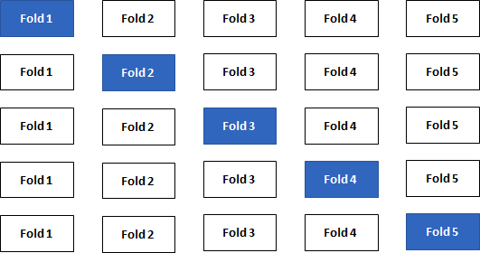
Repeating the split-sample approach several times with different combinations of training/test sets leads to an even better accuracy approximation of your model. The data is split into k folds and one at a time is used as the validation set (“k-Fold Cross-Validation”). State-of-the-art machine learning packages provide this important technique.
Statistical Measures
From now on, I will assume that the k-Fold Cross-Validation is the standard validation method used to calculate certain measures.
1. Regression Models
The regression model with \(\small{ N }\) observations and \(\small{ I }\) columns/variables is
\[\displaystyle{y}_{{n}}=\beta_{{0}}+\beta_{{1}}{x}_{{n}}{1}+\cdots+\beta_{{i}}{x}_{{n}}{i}+ε_{{n}}\]
or in matrix notation
\[\displaystyle{y}={X}\beta+\varepsilon\]
Let \(\small{ \hat{y} }\) denote the fitted value (or prediction value) of \(\small{ y }\) given the estimates \(\small{ \hat{\beta}_{{{1}..{i}}} }\) of \(\small{ {\beta}_{{{1}..{i}}} }\) .
Then
\[\displaystyle{\hat{y}}=\hat{\beta} _{{0}}+\hat{\beta}_{{1}}{x}_{{1}}+\cdots+\hat{\beta}_{{i}}{x}_{{i}}\]
or in matrix notation, the vector of fitted values \(\small{ \hat{y} }\) is calculated by the \(\small{ \displaystyle{N}\times{I} }\) matrix (with \(\small{ N }\) observations and \(\small{ I }\) features) times the vector of estimates \(\small{ \hat{\beta} }\)
\[\hat{y}=X\hat{\beta}\]
with the residuals (error terms)
\[\displaystyle{\varepsilon}=\hat{y}-{y}\]
In order to get a better understanding of the error terms, I visualised a data set with blood pressure depending on the age of a person. The library ggplot2 provides powerful graphs for visualisation.
#create coordinates for our data frame df
   ggplot(df, aes(x=Age,y=Blood_Pressure)) +
      #add data points y~x
         geom_point(color="black") +
      #add regression line
         geom_smooth(method='lm', se=F, color="#d83c2d") +
      #add vertical arrows
         geom_segment(aes(x = Age, y = Blood_Pressure, xend = Age, yend = fitted(model)),
         color="#4e4e4e", size=0.4, arrow = arrow(length = unit(0.2, "cm")))
This R code gives the following plot:
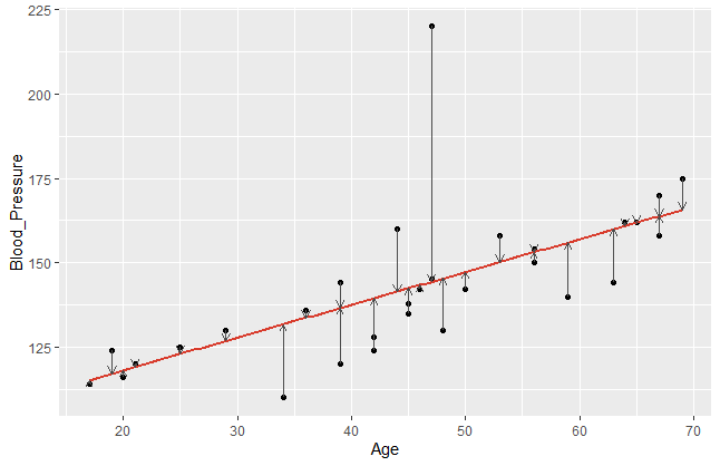
The error terms are visualised by the vertical arrows. It becomes obvious that a model does have a better fit if the data points are closer to the estimated regression line. Comparing different regression models, we take a closer look on these error terms. Since the sign of our \(\small{\varepsilon_{n} }\) can be positive or negative, we usually square it. Hence, let us denote the mean square error of a regression model with \(\small{ n }\) observations as
\[MSE=\frac{1}{N}\sum_{n=1}^{N}\left({\hat{y}}_n-y_n\right)^2\]
This measure can now be compared between different regression models. We assume, that smaller MSE tend to achieve a better prediction accuracy.
2. Classification Models
In comparison to regression, a classification model predicts a discrete target variable, e.g. 0 or 1. However, learning algorithms will give you a probability for each class and now it’s up to the data scientist to choose a threshold parameter (or cut-off point) \(\small{\omega\ \epsilon\ (0\ ,\ 1) }\).
Brier Score
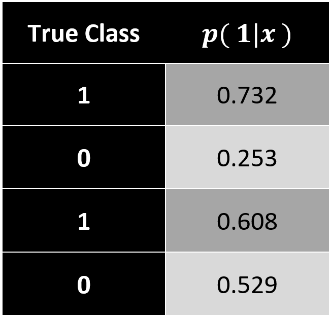
In this case, we can apply a measure that we already know. Analogous to the mean square error (MSE) in regression models, the Brier Score calculates a classification MSE based on probabilities.
\[Brier\ Score=\frac{1}{N}\sum_{n=1}^{N}\left[p\left(class_j|x_n\right)-y_n\right]^2\]
The accuracy of a classification assesses how well your model has split your objects (data points) into the predefined target groups. It is obvious that a good model classifies new data with as little classification error as possible. Errors occur when your model classifies false positive or false negative values.
\[Classification\ Error=\frac{false_{positive}+false_{negative}}{number\ of\ objects}\]
The results of your classification model are often presented in a confusion matrix with a chosen cut-off rate (e.g. \(\small{ \omega=0.6)}\).
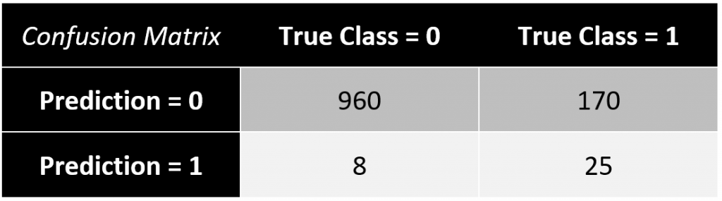
In this example, the classification error equals to \(\small{ 17.49\% }\).
\[\frac{8+170}{960+25+8+25}=\frac{178}{1018}\approx17.49\%\]
A drawback of this measure is a limited explanatory power, since you only consider a single guess of the cut-off rate \(\small{ \omega }\) based on your training data. Therefore, I want to introduce the Receiver Operating Characteristic Curve (ROC curve). It’s a more sophisticated way to assess your prediction model considering all possible cut-off rates. The ROC curve plots the false positive rate (\(\small{ 1-specificity }\)) on the \(\small{ x }\)-axis and the true positive rate (\(\small{ sensitivity }\)) on the \(\small{ y }\)-axis.
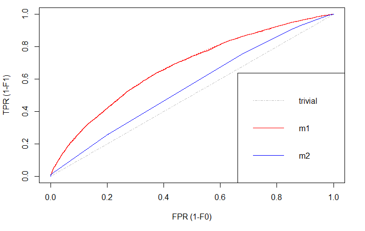
There is always a naïve benchmark in classifying objects into two groups. By the law of large numbers, a completely random classifier will reach a correct classification of \(\small{ 50\% }\). Thus, we only consider prediction models that are better than this benchmark. Otherwise it would be better to apply no model at all and just do random guessing.
Of course, we are interested in those models that differ significantly in correct classification from the trivial result. The blue line shows a logistic regression model and the red line is a decision tree. Both lines are above the trivial benchmark. The sweet spot in this graph lies at (\(\small{ x=0, y=1 }\)) which is the top left edge. At this point the model is almost perfect. Under real world circumstances, this point will never be reached, but the model can come extremely close.
Comparing \(\small{ m1 }\) (decision tree) and \(\small{ m2 }\) (logit model), the ROC curve indicates better results with the decision tree. That is, because this line is above the other.
Area under the ROC curve (AUC)
While comparing plots can be quite hard and inefficient, the ROC curve can be represented in a single measure. By computing the area under the ROC curve (AUC) we still have the information which curve lies above the other, since this area will be greater, but we also have a complete summary within just one numeric value. The AUC of different models can easily be compared by humans or machines.
Linear Regression #8: Linearity
Very often in order to come closer to the “true” model, regression models contain non-linear terms. In 1969 James Ramsey developed the Regression Equation Specification Error Test (RESET) as a general specification test. It examines whether non-linear combinations of the fitted values explain the target variable.
Linear Model:
\[H_0:\ \mathbb{E}\left[y_i\middle|\ x_i\right]=x_i\beta\]
Non-Linear Model:
\[H_1:\ \mathbb{E}\left[y_i\middle|\ x_i\right]\neq x_i\beta\]
The procedure of testing is described hereafter:
- Build the standard OLS linear regression model.
- Use the fitted values of the linear regression and add them to a new model. Set \(\small{ K }\) (often \(\small{ K=1,2,3 }\) )
\[{\hat{y}}_{RESET}=x_i\beta+\sum_{k=1}^{K}\omega_k\ {\hat{y}}^{k+1}\] - Use the common F-test to decide if \(\small{ {H_0:\ \omega}_{1..K}=0 }\).
- If \(\small{ H_0 }\) is rejected, the linear model is misspecified and hence there are non-linear terms.
In R, the test can be run by the command \(\small{ resettest(model) }\).
Linear Regression #7: Normal Distribution
When applying OLS regression or related statistics (e.g. F-test), there are certain assumptions that are essential for a robust and unbiased model. The normality assumption is one of them. We expect the error terms to be normally distributed. In many cases, outlying data points are the reason for non-normality.
There are many graphical ways to identify non-normality with plots. For instance, QQ-plots show the empirical quantiles vs. the theoretical quantiles of a normal distribution. The better our empirical data points fit the red line, the closer is our data to a normal distribution.
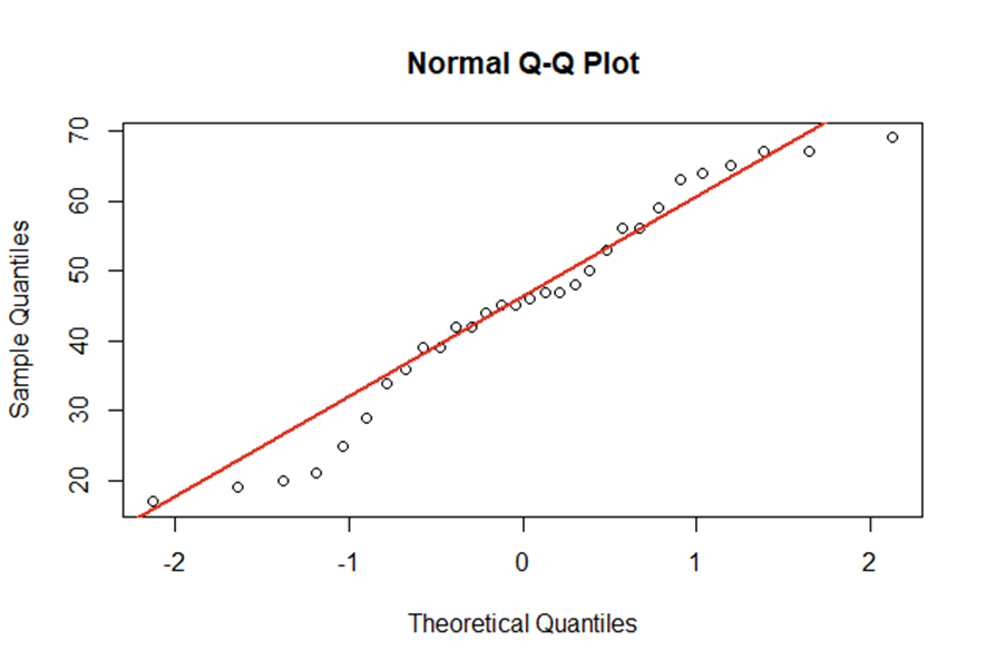
As already shown, visualisations are perfect for getting a first overview of the data. However, you should also consider test statistics with \(\small{ H_0:\ \varepsilon_i\sim N }\) and \(\small{ H_1: \varepsilon_i\sim D_0\neq\ N }\).
Two important test statistics are the Kolmogorov-Smirnow test and the Jarque-Bera test.
Linear Regression #6: Heteroscedasticity
Tests for Heteroscedasticity
For basing inference on OLS, the error terms need to be homoscedastic. That is a constant variance of the error terms. Again, we can apply graphical methods in order to get a first overview. Therefore, we plot the studentised residuals vs. the fitted values and examine the distribution of the data points. If there is an increase in variance, there might be heteroscedasticity.
White Test
The White test for heteroscedasticity has the following hypotheses:
\[H_0:\ \mathbb{E}\left[\varepsilon_i^2\middle|\ X_i\right]=\sigma^2=const\]
\[H_1:\ \mathbb{E}\left[\varepsilon_i^2\middle|\ X_i\right]=\sigma_i^2\neq\sigma_{k\neq i}^2\neq const\]
The null hypothesis assumes that the error terms all have the same constant variance. The alternative hypothesis on the contrary assumes that there are differences between the variances of the error terms and they are hence not constant.
With a regression model \(\small{ \hat{y}=X\hat{\beta} }\), the White test procedures as follows:
- Extract the residuals \(\small{ {\hat{\varepsilon}}_i }\) and square them: \(\small{ {\hat{\varepsilon}}_i^2 }\)
- Run auxiliary regression \(\small{ {\hat{\varepsilon}}_i=\beta_0+\beta_1x_1+\ldots+\beta_nx_n }\).
Idea: If there is heteroscedasticity, then \(\small{ \mathbb{E}\left[\varepsilon_i^2\middle|\ x_i\right] }\) depends on \(\small{ x_i }\) and thus \(\small{ x_i }\) influences \(\small{ \varepsilon_i^2 }\). - Let \(\small{ N }\) be the number of observations and \(\small{ R_{aux}^2 }\) the R-Squared of the auxiliary regression model.
- Calculate the test statistic \(\small{ \theta=N\ast\ R_{aux}^2 }\) and test whether \(\small{ \theta }\) follows the \(\small{ \mathcal{X}_q^2 }\)-distribution with \(\small{ q }\) degrees of freedom or not.
\(\small{ H_0:\theta\sim\mathcal{X}_q^2 }\) or \(\small{ H_1:\theta\sim\mathcal{D}\neq\mathcal{X}_q^2 }\)
R-Code: Manual White Test for Heteroscedasticity
# Extract Squared Residuals
res=lr$residuals
res2=res^2

# Run Auxiliary Regression
aux=lm(res2~df$X)

# Calculate Test Statistic
N=length(res)
R2=summary(aux)$r.squared
theta= N*R2

# Testing Result
p_value <- 1 - pchisq(theta, N-1)
if(p_value>0.05){
  print("Homoscedasticity, accept H0!")
}
else{
  print("Heteroscedasticity, reject H0!")
}
Conclusion
If we detect heteroscedasticity, the Gauss-Markow assumptions are violated. Hence, we cannot apply OLS regression, but have to use FGLS instead:
Homoscedasticity
\[Var\left(\hat{\beta}\middle|\ X\right)\\=\left(X^\prime X\right)^{-1}\left[X^\prime \ Var\left(\varepsilon\middle|\ X\right)X\right]\left(X^\prime X\right)^{-1} \]
Heteroscedasticity
\[Var\left(\hat{\beta}\middle|\ X\right)\\=\left(X^\prime X\right)^{-1}\left[X^\prime\sigma^2I_NX\right]\left(X^\prime X\right)^{-1}\\=\sigma^2\left(X^\prime X\right)^{-1} \]
Linear Regression #5: Residual Analysis
Whenever building a regression model, we have certain assumptions (e.g. Gauss-Markow theorem). For instance, a normal distribution of the error terms is essential for OLS regression. We use model diagnostic statistics or graphs in order to detect problems or errors in our modelling.
Residual Analysis
In a regression model, we call the difference between the fitted values and the observed target values the residuals.
\[e=\hat{y}-y=X\hat{\beta}-y=\left(I-P\right)y\]
\[= My \sim \left(0,\ \sigma^2\left(I-P\right)\right)\]
where \(\small{M=I-P}\) is the residual maker and \(\small{P=X\left(X^\prime X\right)^{-1}X^\prime}\) is the projection (“hat”) matrix.
A residual analysis can help us to identify outliers, check for linearity, normality, homoscedasticity or time series properties. For checking, we transform the residuals in a standardised form. The most important transformation was established by Student:
Studentised Residuals
\[t=\frac{e}{\hat{\sigma}\sqrt{1-p_{ii}}}\]
where \(\small{p_{ii} }\) is the \(\small{ i }\) -th diagonal element in the hat matrix and \(\small{ \hat{\sigma} }\) is an appropriate estimate of the variance.
There are two options to calculate the variance of the residuals. The internal studentisation estimates the residual variance based on all observations:
\[{\hat{\sigma}}^2\ =\frac{e^\prime e}{N-K}=\frac{1}{N-K}\sum e_j^2\]
However, if the \(\small{ i }\) -th case is suspected to have a high leverage effect and hence might be an outlier, the external studentisation excluded the \(\small{ i }\) -th observation in order to calculate the variance only based on the other observations.
\[{\hat{\sigma}}_{-i}^2\ =\frac{{(e}_{-i})^{\prime} e_{-i}}{N-K-1}=\frac{1}{N-K}\sum e_{j\neq i}^2\]
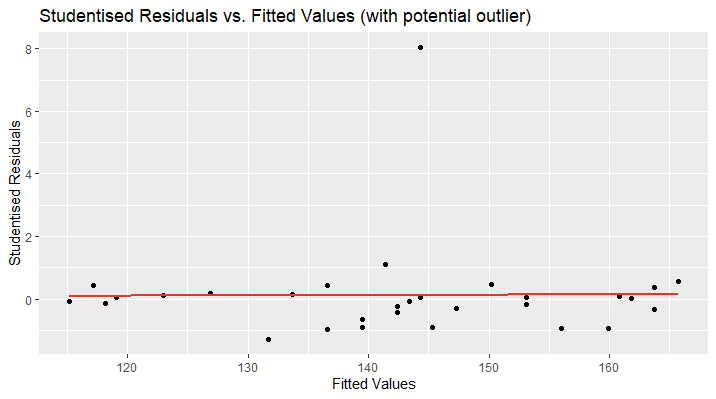
By plotting the studentised residuals against the fitted values, the occurrence of heteroscedasticity can be graphically seen. Moreover, hints for normal distribution and linearity are visible.
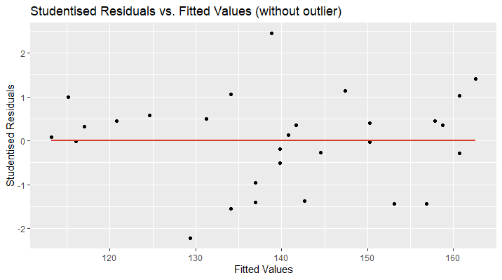
Let’s take a look at an example. The following plot shows the studentised residuals of a linear model’s prediction of the blood pressure based on the age of a person. The plot looks distorted and we discover a data point far away from the other observations. We can suspect this data point to be a potential outlier. The red line shows the studentised regression line and should be located at approximately \(\small{ y=0 }\) and the data points closely above and below.
In the second plot, I have removed the outlying data point and now, the regression line perfectly fits the x-axis ( \(\small{ y=0 }\) ). Furthermore, the data points are randomly located above and over the red curve, which is a sign for linearity. There might be an increase in the variance of the studentised residuals as the fitted values increase. This could be a hint for heteroscedasticity and more tests need to be applied.
The R code for this visualisation is as follows:
# Delete Outlier
df.new=df[-2,]

# Train Linear Model
lr.new=lm(Blood_Pressure ~., data=df.new)

# Visualise with ggplot2
ggplot(lr.new, aes(x=lr.new$fitted.values,y=rstudent(lr.new)))
   + geom_point(color="black")
   + geom_smooth(method='lm', se=F, color="#d83c2d")
   + ggtitle("Studentised Residuals vs. Fitted Values (without outlier) ")
   + xlab("Fitted Values") + ylab("Studentised Residuals")
Formal Tests for Outliers
After considering outlier detection by visualisation of the data, we now want to identify outliers by formal statistical measurements.
The Leverage Effect
The leverage effect of a data point is given by \(\small{ 0\le\ pii\le1 }\) , which is the \(\small{ i }\)-th diagonal element of the hat matix. In R the \(\small{p_{ii} }\) can be calculated by the function \(\small{ hatvalues(model) }\) . The higher the value of the leverage, the higher will be the effect of this observation on the regression coefficients. First conclusions can therefore be drawn by identifying data points with higher leverage compared to the other observations. As a rule of thumb, in cases of \(\small{ p_{ii}>\frac{2K}{N} }\) the data points need further examination.
The Mahalanobis Distance
An important numerical method to detect outliers is the squared Mahalanobis distance. It considers the depending or surrounding variables in context and measures the distance between the j-th observation and the center of the distribution.
\[D^2\ =\ \left(x_j\ -\ \mu\right)^\prime\ \mathrm{\Sigma}^{-1}\left(x_j\ -\ \mu\right)\]
with the covariance matrix \(\small{ \mathrm{\Sigma} }\).
The Cook’s Distance
The Cook’s distance answers the question, how much influence is caused by the \(\small{i }\)-th data point in our regression model.
\[C_i=\frac{\left(\hat{y}-{\hat{y}}_{-i}\right)^2}{K{\hat{\sigma}}^2}=\frac{\varepsilon_i^2}{K{\hat{\sigma}}^2}\ast\left[\frac{p_{ii}}{1-p_{ii}}\right]\]
where \(\small{ {\hat{\sigma}}^2\ =\frac{e^\prime e}{N-K}=\frac{1}{N-K}\sum e_j^2 }\) . As a rule of thumb, the \(\small{ i }\)-th data point has a large influence if \(\small{ C_i>\frac{4}{N} }\).
Data Science #4: Data Preprocessing
The first thing when obtaining new data is getting familiar with the structure. That is for instance, the meaning, scaling and distribution of variables, the number of observations and potential relationship or dependencies between columns or rows. General measures of statistics (mean, median, interquartile range) can be useful.
Data Selection
The selection of data depends on the business question or the objective of the model. If possible, the raw data should be as clean as possible. In general, the more observations you can get, the more possibilies you will have in the modelling process. You can always select a sub-sample. However, if you have only few observations to train your model on, then you might accept certain limitations of the resulting model.
Cleaning Data
Before training any model, it is vital to reduce noise in the data set. This noisiness is caused by errors, missing values or outliers. Hence, the detection and a proper treatment influences the outcome of your prediction significantly. Concerning errors in your data, so far we can say: Correct the error values if feasible or else treat them as missing values as follows.
Missing Values
One of the first things during data preprocessing is identifying missing values. We can simply achieve this by finding empty cells in our tabular data df:
sapply(df, function(x) sum(is.na(x)))
Sometimes it might not be as easy as finding empty cells depending on the data source. Often missing values are decoded by the researcher with some specific value (e.g. “9” or “999”). Useful commands in R to identify those values are
table(df$columnX)
and
hist(df$columnX)
While dealing with missing values the data scientist can follow different approaches. If there is a large data set with only few missing values, it might be comfortable to just delete all incomplete observations.
df <- na.omit(df$columnX)
However in most cases this cleaning method is unsuitable because too much information is lost. Sometimes even missing values have a special meaning. In this case we could add a dummy variable containing the information whether a value was missing or not.
df$newDummyCol = ifelse(is.na(df$columnX),1,0)
After storing this information, the column with the missing values can be edited. The data scientist makes use of various imputation techniques. That is estimating the missing values and filling in a proper estimate for every single observation. A very naïve strategy would be replacement by the mean or median of the complete observations.
df$columnX[is.na(df$columnX)] = mean(df$columnX[!is.na(df$columnX)])
More sophisticated methods are linear regressions or decision trees based on the other features/variables
regr =lm(columnX~colY+colZ, data=df[!is.na(df$columnX),])
df$columnX[is.na(df$columnX)]=predict(regr, newdata = df[is.na(df$columnX),])
There are also some packages that can do this process very conveniently.
Outlier Detection
Outlying values are a big issue in data preprocessing. Here, we speak of values that are located far too distant from most other observations. Thus, they might have a misleading effect on the predictions and cause biases or high variance.
The detection of outliers can be obtained by visualisation using histograms or boxplots and by numerical approaches. A simple z-transformation helps to standardise/normalise the data in order to get a better overview on the distribution
\[z_j=\frac{x_j-\mu}{\sigma}\]
where \(\small{ \mu }\) is the mean and \(\small{ \sigma }\) the standard deviation. In R we apply this by
df$columnX = standardize(df$columnX)
We assume that outlying values have z-values larger than 3 or smaller than -3.
Another numerical method to detect outliers is the squared Mahalanobis distance. In addition to the previous z-transformation, the squared Mahalanobis distance does also consider the depending or surrounding variables in context. Hence, this is an even better technique.
\[D^2\ =\ \left(x_j\ -\ \mu\right)^\prime\mathrm{\Sigma}^{-1}\ \left(x_j\ -\ \mu\right)\]
with the covariance matrix \(\small{ \mathrm{\Sigma} }\).
The treatment of outliers resembles the missing value treatment. If these outliers are no errors, it might be possible to keep them in the data set. Otherwise imputation techniques like mean replacement or linear regression can be applied. In some cases, it might even be sensible to exclude the outlying observations.
Data Transformation
Now having a nice clean data set, you should still not start building your prediction model. Depending on the model type you are using, the transformation of certain variables is necessary in order to increase the performance and accuracy levels of predictions.
Feature Scaling
When it comes to different algorithms, you as a data scientist must consider different requirements. Many models use the Euclidean distance measure between two data points. Hence, they struggle with different scaling of the variables. Especially machine learning algorithms (e.g. k-nearest-neighbors) can reach much better performances when the features are normalised/standardised.
Models that use linear or logistic regression follow the Gauss-Markov-theorem and will (by definition) always give the best linear unbiased estimator (BLUE). That is giving weights to the features automatically. In other words, we don’t have to scale our variables when using linear or logistic regression techniques, but it helps the data scientist to interpret the resulting model. With normalised features, the interpretation of the intercept will be the estimate of \(\small{ y }\) when all regressors \(\small{ x_i }\) are set to their mean value. The coefficients are now in units of the standard deviation. Furthermore, scaling can reduce the computational expense of your model training.
Another set of algorithms, that are completely unaffected by scaling of features are all tree-based learners. But even when you use a decision tree, there is a good reason for normalising your data: You leave the door open to add other learning algorithms for comparison or ensemble learning.
Unsupervised Binning/Distrecisation
The process of aggregating data into groups of higher level of abstraction is called binning (for two groups) or discretisation (for more than two groups). Based on their value, the data is put into classes representing hierarchies. For instance, a person’s height is a continuous variable and can be assigned to dicrete groups “small”, “medium” and “large”. Although some information is lost in this process, you achieve a much cleaner data set with less noise. In most cases, you achieve a more robust prediction model. The number of groups can be chosen by the data scientist.
library("recipes")
d = discretize(df$columnX, cuts=3, min_unique=0, na.rm=TRUE)
df$columnXdiscr = predict(d, new_data = df$columnX)
Supervised Discretisation
The term “supervised” is always the hint for labelled data (including the outcome or target value). As an initial step, the target variable can be used to discretise a feature. This method can be used in order to maximise the information gain of discretisation for your prediction.
Feature Engineering
The topic of feature engineering is essential for modern machine learning. It is both difficult and expensive, since the data scientist needs to perform most part of it manually. Our goal is to change or create new features with a higher explanatory character than the raw data could offer.
In most cases, lots of experience and theoretical background are needed in order to understand the relationship between different variables.
a. Aggregations
The simplest way of feature engineering is a basic aggregation of data. That can be obtained by discretisation techniques (already mentioned above).
b. Transformation of Distribution
There are different famous transformation techniques in order to change the distribution of the data. Assume a variable contains both small numeric values and some large values. Here, we can apply a simple log-transformation to lower the larger values and hence tighten the distribution. Another example is the Box-Cox-transformation.
Often the goal is to achieve a more normal distribution, since many learning algorithms (e.g. Regression) need that normal assumption.
c. Trend variables
When it comes to time series, an important feature can be the marginal difference between two data points. This can give us an absolute trend \(\small{ \frac{x_t-x_{t-i}}{i} }\) or a relative trend \(\small{ \frac{x_t-x_{t-i}}{x_{t-i}} }\).
d. Weight of Evidence (WOE)
The weight of evidence (WOE) is a powerful transformation of a discrete (categorical) feature into a numerical measure describing the good or bad influence of this category on the target variable (information value).
\[WOE_i=\ln{\left(\frac{p\left(GOOD\right)_i}{p\left(BAD\right)_i}\right)}\]
where
\[p\left(GOOD\right)_i=\frac{absolute\ number\ of\ GOODs\ in\ category\ i}{total\ number\ of\ GOODs\ in\ all\ categories\ 1..i}\]
On the training data we can calculate the WOE in R using the library InformationValue:
#load library
library(“InformationValue”)

#calculate and add column of WOEs on labelled data set (train data)
df$columnXwoe=WOE(df$columnXdiscr, df$target, valueOfGood = 1)

#calculate and store WOE table to merge with unlabelled new data
woe.table.colX=WOETable(df$columnXdiscr, df$target, valueOfGood = 1)
Remember to store the WOETable for later merging with unlabelled new data sets:
tmp=as.data.frame(df$columnXdiscr)
colnames(tmp)="CAT"
tmp$row=rownames(tmp)
tmp2=(merge(tmp, woe.table.colX))
tmp2$row=as.numeric(tmp2$row)
df$columnXwoe =tmp2[order(tmp2$row),]
remove(tmp,tmp2)
Feature Selection
It is often not to difficult to create a large variety of features and transformations of the data. However, in the end the best transformation techniques might add only little explanatory power to the machine learning model. Therefore, a proper selection of features needs to be performed before building the model with too many (maybe unimportant) features. The curse of dimensionality is often mentioned in this context. The more different features we add to our model, the more dimensions are used and hence the model becomes more complex. The problem of a more complex model can be a high variance when applying it. Another difficulty of many features is the cost of time and computing power for training the model.
A proper set of features can be obtained by different approaches:
a. Filter Approach
A statistical indicator for variable importance is given by a high (or at least moderate) correlation between a feature and the target variable. Depending on the scaling of the variables, a suitable correlation measures is taken into account (e.g. Pearson, Fisher,…).
The filter approach assesses only one feature at a time and does not consider the interaction between different explanatory features. Therefore, the filter approach is less effective than the following method.
b. Wrapper Approach
A more considerate way to select features is the wrapper approach, that also considers the relationship between the all selected features. This is done iteratively by comparing all possible \(\small{ 2^{n}-1 }\) models containing up to a maximum of \(\small{ n }\) explanatory variables.
The selection can be achieved by forward, backward or stepwise selection. For instance, the forward selection starts with only one feature and iteratively adds one more feature which adds the most explanatory power to the model. This process is stopped as soon as a predefined threshold of marginal accuracy added to the model is not passed anymore.
Using the wrapper approach usually gives a better performance, but also takes more computational cost.
Linear Regression #4: Model Selection Criteria
We define a criterion \(\small{ C(m) }\) that measures the quality of a model \(\small{ m }\) . In general, we need to find the model \(\small{ m^{*} }\) that minimises the selection criterion \(\small{ C(m) }\) for all possible \(\small{ m }\) .
For beginning, let us recall the mean squared prediction error ( \(\small{ MSPE }\) ) for our model \(\small{ m }\) . The MSPE is the expected value of the squared difference between the fitted values (prediction) \(\small{ {\hat{y}}_{i}\left(m\right) }\) and the values of the unobservable function \(\small{ y_i^\ast }\) .
\[MSPE(m)=\frac{1}{N} \sum_{i=1}^N E[(\hat{y}_i (m)-y_i)^2]\]
The MSPE contains information about the model bias, the estimation error and the variance. With an increasing number of included features \(\small{ \left|m\right| }\) , the model bias will decrease and the estimation error increase. An estimation of the \(\small{ MSPE }\) can be given by
\[\widehat{MSPE}\left(m\right)=\frac{1}{N}RSS\left(m\right)+2\frac{\left|m\right|}{N}{\hat{\sigma}}^2\]
where \(\small{ RSS=N\ast\ MSE=\sum\nolimits_{i=1}^{N}\left({\hat{y}}_i\left(m\right)-y_i\right)^2 }\) . The increasing number of variables \(\small{ \left|m\right| }\) is used as a “punishment” or penalty. As the number of included features grows, the higher will be the value of the selection criterion and hence this model is not being preferred. This prevents overfitting. Collin Mallows later proposed a normalised version of this criterion:
\[C_p\left(m\right)=\frac{RSS\left(m\right)}{{\hat{\sigma}}^2}-N+2\left|m\right|\]
Both criteria lead to the same optimal model \(\small{ m }\) .
Cross Validation Criteria
Alternatives to the MSPE are cross-validation criteria:
\[CV(m)=\frac{1}{N}\sum_{i=1}^{N}\left({\hat{y}}_{-i}(m)-y_i\right)^2\]
This criterion is the mean squared difference between the true value \(\small{ y_i }\) and the prediction \(\small{ {\hat{y}}_{-i}\left(m\right) }\) trained on a data set without the \(\small{ i }\) -th point. Thus, it is called a leave-one-out estimator.
Generalised Information Criterion
An important measure of model selection is the generalised information criterion ( \(\small{ GIC }\) ).
\[GIC\left(m\right)=\ln{\left({\widetilde{\sigma}}^2\left(m\right)\right)}+a_N\frac{\left|m\right|}{N}\]
The \(\small{ GIC }\) is based on the logarithm of the maximum-likelihood estimator \(\small{ {\widetilde{\sigma}}^2\left(m\right) }\) .
We can derive two special cases of the \(\small{ GIC }\) that are very popular among statisticians.
1. Akaike Information Criterion (AIC)
The Akaike Information Criterion sets \(\small{ a_N=2 }\) in the \(\small{ GIC }\) formula. Thus, we have
\[AIC\left(m\right)=\ln{\left({\widetilde{\sigma}}^2\left(m\right)\right)}+2\frac{\left|m\right|}{N}\]
When using OLS regression, the maximum likelihood estimator for the variance of a model’s residuals distributions is \(\small{ {\widetilde{\sigma}}^2\left(m\right)=RSS/N }\) , where \(\small{ RSS }\) is the residual sum of squares.
\[AIC_{OLS}\left(m\right)=\ln{\left(\frac{RSS}{N}\right)}+2\frac{\left|m\right|}{N}\]
The \(\small{ AIC }\) criterion is asymptotically optimal under certain conditions. As well, as \(\small{ CV }\) , \(\small{ Cp }\) and \(\small{ MSPE }\) . However, \(\small{ AIC }\) is not consistent. Under the assumption that the “true model” is not in the candidate set, we are interested in the unknown “oracle model” \(\small{ m^\ast }\) . As \(\small{ N\rightarrow\infty }\) ,
\[\frac{\left|\left|g-\hat{y}\left(\hat{m}\right)\right|\right|^2}{\left|\left|g-\hat{y}\left(m^\ast\right)\right|\right|^2} \rightarrow m_{true}\]
Moreover, the \(\small{ AIC }\) is asymptotically equivalent to the leave-one-out \(\small{ CV }\) criterion.
2. Baysian-Schwarz Information Criterion (BIC)
The Akaike Information Criterion sets \(\small{ a_N=\ln(N) }\) in the \(\small{ GIC }\) formula. Thus, we have
\[BIC\left(m\right)=\ln{\left({\widetilde{\sigma}}^2\left(m\right)\right)}+\ln(N)\frac{\left|m\right|}{N}\]
Again, when using OLS regression, the maximum likelihood estimate for the variance of a model’s residuals distributions is \(\small{ {\widetilde{\sigma}}^2\left(m\right)=RSS/N }\) , where \(\small{ RSS }\) is the residual sum of squares.
\[BIC_{OLS}\left(m\right)=\ln{\left(\frac{RSS}{N}\right)}+\ln(N)\frac{\left|m\right|}{N}\]
The BIC Criterion is consistent. However, it is not asymptotically optimal. As \(\small{ N\rightarrow\infty }\) ,
\[\hat{m} \rightarrow m_{true}\]
Linear Regression #3: Variable Selection
In Econometrics and Data Science, a necessary procedure in building a prediction model is validation. I already presented the most common techniques of model validation in this article.
Let us now have a deeper look on these methods from statistical perspective. For robust prediction models it is vital to split the data with \(\small{ N }\) observations into two different sets. The train set with \(\small{ n_1<N }\) rows and the test/validation set with \(\small{ n_2=N-n_1 }\) rows.
Now, we build the regression model with the training data. Using the mean-square-error, we afterwards evaluate the regression model based on the untouched test data.
\[MSE=\frac{1}{n_2}\sum_{i=n_1+1}^{N}\left({\hat{y}}_i-y_i\right)^2\]
We choose the model that minimises the MSE for our validation set.
I have also described the procedure of feature selection from a data scientist’s perspective in this aricle.
Sequential Variable Selection
There are basically four different algorithms or procedures for selecting variables to include in the model.
Forward Selection
Starting from a minimum set of variables based on economic theory, the algorithm determines which regressor (not yet included) reduces most the RSS in the regression model. The algorithm iteratively adds variables until a stopping criterion is met. That is when \(\small{\Delta RSS < \tau }\), where \(\small{ \tau }\) is a threshold metric to avoid adding variables with little or no reduction of RSS.
Backward Elimination
The other way around, the algorithm starts with the whole set of variables and iteratively excludes features that add little or no reduction of RSS to the model.
Stepwise Selection
The combination of forward and backward selection. The algorithm can add and exclude variables at each iteration.
Random variable selection
Often neglected in traditional statistic theory, but nowadays becoming very popular in famous machine learning algorithms, a random selection of variables can provide a proper prediction model. Though this method is only used in combination with many different individual random models in a composite ensemble model.