

Whenever building a regression model, we have certain assumptions (e.g. Gauss-Markow theorem). For instance, a normal distribution of the error terms is essential for OLS regression. We use model diagnostic statistics or graphs in order to detect problems or errors in our modelling.
Residual Analysis
In a regression model, we call the difference between the fitted values and the observed target values the residuals.
\[e=\hat{y}-y=X\hat{\beta}-y=\left(I-P\right)y\]
\[= My \sim \left(0,\ \sigma^2\left(I-P\right)\right)\]
where \(\small{M=I-P}\) is the residual maker and \(\small{P=X\left(X^\prime X\right)^{-1}X^\prime}\) is the projection (“hat”) matrix.
A residual analysis can help us to identify outliers, check for linearity, normality, homoscedasticity or time series properties. For checking, we transform the residuals in a standardised form. The most important transformation was established by Student:
Studentised Residuals
\[t=\frac{e}{\hat{\sigma}\sqrt{1-p_{ii}}}\]
where \(\small{p_{ii} }\) is the \(\small{ i }\) -th diagonal element in the hat matrix and \(\small{ \hat{\sigma} }\) is an appropriate estimate of the variance.
There are two options to calculate the variance of the residuals. The internal studentisation estimates the residual variance based on all observations:
\[{\hat{\sigma}}^2\ =\frac{e^\prime e}{N-K}=\frac{1}{N-K}\sum e_j^2\]
However, if the \(\small{ i }\) -th case is suspected to have a high leverage effect and hence might be an outlier, the external studentisation excluded the \(\small{ i }\) -th observation in order to calculate the variance only based on the other observations.
\[{\hat{\sigma}}_{-i}^2\ =\frac{{(e}_{-i})^{\prime} e_{-i}}{N-K-1}=\frac{1}{N-K}\sum e_{j\neq i}^2\]
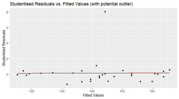
By plotting the studentised residuals against the fitted values, the occurrence of heteroscedasticity can be graphically seen. Moreover, hints for normal distribution and linearity are visible.
Let’s take a look at an example. The following plot shows the studentised residuals of a linear model’s prediction of the blood pressure based on the age of a person. The plot looks distorted and we discover a data point far away from the other observations. We can suspect this data point to be a potential outlier. The red line shows the studentised regression line and should be located at approximately \(\small{ y=0 }\) and the data points closely above and below.
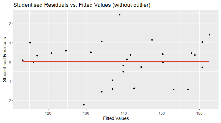
In the second plot, I have removed the outlying data point and now, the regression line perfectly fits the x-axis ( \(\small{ y=0 }\) ). Furthermore, the data points are randomly located above and over the red curve, which is a sign for linearity. There might be an increase in the variance of the studentised residuals as the fitted values increase. This could be a hint for heteroscedasticity and more tests need to be applied.
The R code for this visualisation is as follows:
# Delete Outlier
df.new=df[-2,]

# Train Linear Model
lr.new=lm(Blood_Pressure ~., data=df.new)

# Visualise with ggplot2
ggplot(lr.new, aes(x=lr.new$fitted.values,y=rstudent(lr.new)))
   + geom_point(color="black")
   + geom_smooth(method='lm', se=F, color="#d83c2d")
   + ggtitle("Studentised Residuals vs. Fitted Values (without outlier) ")
   + xlab("Fitted Values") + ylab("Studentised Residuals")
Formal Tests for Outliers
After considering outlier detection by visualisation of the data, we now want to identify outliers by formal statistical measurements.
The Leverage Effect
The leverage effect of a data point is given by \(\small{ 0\le\ pii\le1 }\) , which is the \(\small{ i }\)-th diagonal element of the hat matix. In R the \(\small{p_{ii} }\) can be calculated by the function \(\small{ hatvalues(model) }\) . The higher the value of the leverage, the higher will be the effect of this observation on the regression coefficients. First conclusions can therefore be drawn by identifying data points with higher leverage compared to the other observations. As a rule of thumb, in cases of \(\small{ p_{ii}>\frac{2K}{N} }\) the data points need further examination.
The Mahalanobis Distance
An important numerical method to detect outliers is the squared Mahalanobis distance. It considers the depending or surrounding variables in context and measures the distance between the j-th observation and the center of the distribution.
\[D^2\ =\ \left(x_j\ -\ \mu\right)^\prime\ \mathrm{\Sigma}^{-1}\left(x_j\ -\ \mu\right)\]
with the covariance matrix \(\small{ \mathrm{\Sigma} }\).
The Cook’s Distance
The Cook’s distance answers the question, how much influence is caused by the \(\small{i }\)-th data point in our regression model.
\[C_i=\frac{\left(\hat{y}-{\hat{y}}_{-i}\right)^2}{K{\hat{\sigma}}^2}=\frac{\varepsilon_i^2}{K{\hat{\sigma}}^2}\ast\left[\frac{p_{ii}}{1-p_{ii}}\right]\]
where \(\small{ {\hat{\sigma}}^2\ =\frac{e^\prime e}{N-K}=\frac{1}{N-K}\sum e_j^2 }\) . As a rule of thumb, the \(\small{ i }\)-th data point has a large influence if \(\small{ C_i>\frac{4}{N} }\).