
The regression model with \(\small{ N }\) observations and \(\small{ I }\) columns/variables is
\[\displaystyle{y}_{{n}}=\beta_{{0}}+\beta_{{1}}{x}_{{n}}{1}+\cdots+\beta_{{i}}{x}_{{n}}{i}+ε_{{n}}\]
or in matrix notation
\[\displaystyle{y}={X}\beta+\varepsilon\]
Let \(\small{ \hat{y} }\) denote the fitted value (or prediction value) of \(\small{ y }\) given the estimates \(\small{ \hat{\beta}_{{{1}..{i}}} }\) of \(\small{ {\beta}_{{{1}..{i}}} }\) .
Then
\[\displaystyle{\hat{y}}=\hat{\beta} _{{0}}+\hat{\beta}_{{1}}{x}_{{1}}+\cdots+\hat{\beta}_{{i}}{x}_{{i}}\]
or in matrix notation, the vector of fitted values \(\small{ \hat{y} }\) is calculated by the \(\small{ \displaystyle{N}\times{I} }\) matrix (with \(\small{ N }\) observations and \(\small{ I }\) features) times the vector of estimates \(\small{ \hat{\beta} }\)
\[\hat{y}=X\hat{\beta}\]
with the residuals (error terms)
\[\displaystyle{\varepsilon}=\hat{y}-{y}\]
We assume that our error terms are normally distributed \(\small{ \displaystyle{\varepsilon}\sim{N}{\left({0},\sigma^{2}{I}_{{N}}\right)} }\) where \(\small{ \displaystyle{I}_{{N}} }\) is the \(\small{ \displaystyle{N}\times{N} }\) identity matrix.
Gauss-Markow-Theorem
According to the Gauss-Markow theorem we make three important assumptions:
- The expectation of the error terms is zero: \(\small{ {E}{\left[\varepsilon\right]}={0} }\)
- The error terms are homoscedastic: \(\small{ \displaystyle{V}{\left[\varepsilon\right]}=\sigma^{2}{I}_{{N}} }\)
- The error terms are uncorrelated: \(\small{ \displaystyle{E}{\left[\varepsilon_{{r}}\varepsilon _{{s}}\right]}={0} }\) for \(\small{ \displaystyle\varepsilon_{{r}}\ne\varepsilon_{{s}} }\)
Ordinary Least Square Estimator (OLS)
Let’s visualise the error terms of a common regression function. In the following example, I plot the blood pressure of patients against their age and visualise the error terms by vertical arrows.
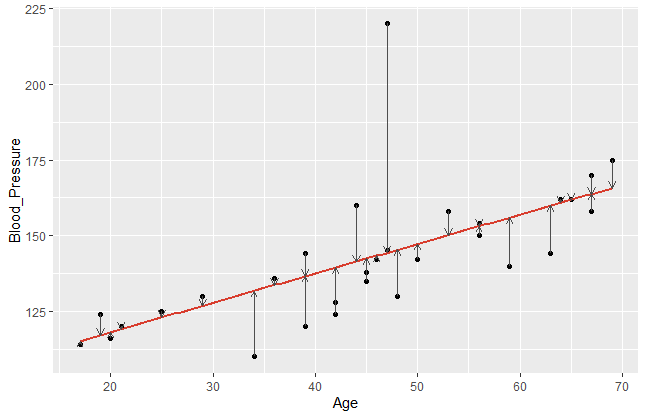
It becomes obvious that a model fits better if the data points are closer to the estimated regression line. Comparing different regression lines, we take a closer look on these error terms. Since the sign of our \(\small{ \varepsilon_n }\) can be positive or negative, we usually square it. Hence, let us denote the sum of squared residuals (SSR) of a regression model with \(\small{ n }\) observations as
\[SSR=\sum_{n=1}^{N}(\hat{y}_n-y_n)^2\]
or in matrix notation
\[\displaystyle\varepsilon ^\prime \varepsilon ={\left({\hat{y}}-{y}\right)} ^\prime {\left({\hat{y}}-{y}\right)}\]
In order to find the best linear unbiased estimator (BLUE), the goal is to minimise the SSR.
\[ \varepsilon^\prime\varepsilon=\left(\hat{y}-y\right)^\prime\left(\hat{y}-y\right) \]
\[ =\left(X\hat{\beta}-y\right)^\prime\left(X\hat{\beta}-y\right) \]
\[ =\left({\hat{\beta}}^\prime X^\prime-y^\prime\right)\left(X\hat{\beta}-y\right) \]
\[ ={\hat{\beta}}^\prime X^\prime X\hat{\beta}-{\hat{\beta}}^\prime X^\prime y-y^\prime X\hat{\beta}+y^\prime y \]
\[ ={\hat{\beta}}^\prime X^\prime X\hat{\beta}-2\ {\hat{\beta}}^\prime X^\prime y+y^\prime y \]
Use the first order condition (FOC) to find the minimum
\[\frac{\partial\varepsilon^\prime\varepsilon}{\partial\hat{\beta}}=2X^\prime X\hat{\beta}-2X^\prime y=0 \]
\[ \Longleftrightarrow\ X^\prime X\hat{\beta}=X^\prime y\]
\[\Longleftrightarrow\hat{\beta}={\left(X^\prime X\right)^{-1}\ X}^\prime y\ \]
Hence, \(\small{ \hat{\beta}={\left(X^\prime X\right)^{-1}\ X}^\prime y }\) is BLUE according to Gauss-Markow with \(\small{ \mathbb{V}\left(\hat{\beta}\right)=\sigma^2\left(X^\prime X\right)^{-1} }\) .
The vector of fitted values \(\small{ \hat{y}=X\hat{\beta}=Py }\) where \(\small{ P=X\left(X^\prime X\right)^{-1}X^\prime }\) is the orthogonal projection matrix onto the column space of \(\small{ X }\) , also called “hat matrix”. \(\small{ P }\) is symmetric and idempotent, which means that \(\small{ P=P^2=P^\prime }\) holds. The residual maker \(\small{ M=\left(I-P\right) }\) is orthogonal to the projection matrix, thus \(\small{ M^\prime P=I }\) .
Under normality, we assume that \(\small{ \hat{\beta}\sim\mathcal{N}\left(\beta,\sigma^2\left(X^\prime X\right)^{-1}\right) }\) , since
\[\mathbb{E}\left[\hat{\beta}|X\right]=\beta\]
\[\mathbb{V}\left[\hat{\beta}|X\right]=\left(X^\prime X\right)^{-1}\ast\ X^{\prime\ }\mathbb{V}\left[\varepsilon|X\right]\ X\ast\ \left(X^\prime X\right)^{-1}\]
\[ \mathbb{V}\left[\hat{\beta}|X\right]=\left(X^\prime X\right)^{-1}\ast\ X^\prime\ \Omega\ X\ast\ \left(X^\prime X\right)^{-1}\]
Where \(\small{ \mathbb{V}\left[\varepsilon|X\right]=\Omega=\sigma^2\Psi }\) and thus \(\small{ \Psi }\) is a positive definite matrix. If \(\small{ \Psi=I_N }\) , then the error terms are homoscedastic and we can simplify our result.
\[\mathbb{V}\left[\hat{\beta}|X\right]=\left(X^\prime X\right)^{-1}\ast\ \sigma^2\ (X^\prime X)\left(X^\prime X\right)^{-1}{=\sigma}^2\left(X^\prime X\right)^{-1}\]
In case that \(\small{ \mathbb{V}(\varepsilon)\neq\sigma^2\ I_N }\) we can define a generalised least square estimator (GLS estimator):
\[{\hat{\beta}}_{GLS}=\left(X^\prime{{\Omega}}^{-1}X\right)^{-1}\ X^\prime {\Omega }^{-1}y \]
The GLS estimator is necessarily to be extended to the FGLS estimator (feasible GLS), for \(\small{ \Omega }\) is in general unknown and needs to be estimated. We expect
\[{\hat{\beta}}_{FGLS}=\left(X^\prime{\hat{\Omega}}^{-1}X\right)^{-1}\ X^\prime \hat{\Omega }^{-1}y \]
where \(\small{ \hat{\Omega} }\) is a constant estimator of \(\small{ \Omega }\) . The FGLS estimator is in general non-linear.