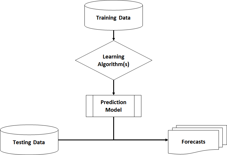
Prediction Models are built on data of the past. A common application is observing a customer’s attributes and behaviour in order to predict whether he will return a purchased item or keep it. Before a model can make such a prediction, it needs to learn from past data that include the outcome label (target variable). After that training process, the model is able to make predictions based on new unlabelled data (=target variable is missing).

Predictive Algorithms
1. Regression Models
Linear or non-linear regression algorithms make predictions/forecasts by calculating a model with a continuous dependent target variable.
Typical business cases are sales predictions or financial forecasts.
2. Classification Models
Classification algorithms classify objects into known groups. (Remember: Groups were unknown in cluster analysis). For instance, a dichotomous target variable might be the risk of credit default (1=default, 0=repayment). At the point of loan application, the outcome is not yet known. However, classification models can make a prediction based on the characteristics/attributes of the applicant (object).
Decision Trees
A decision tree is a set of splitting rules that predicts discrete (classification) or continuous (regression) outcomes. It can be visualised as directed tree-like graph starting from a root node, including various splitter nodes and ending with the possible outcomes (leaves).
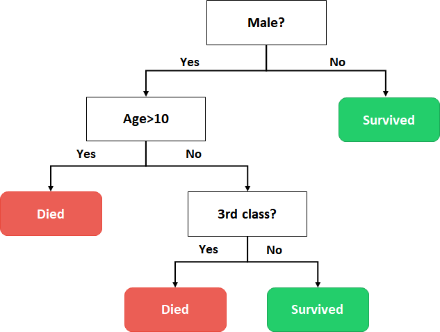
I want to show you two simple examples of decision trees. First, a classification decision tree that classifies the passengers of the Titanic into two groups: survivors and fatalities.

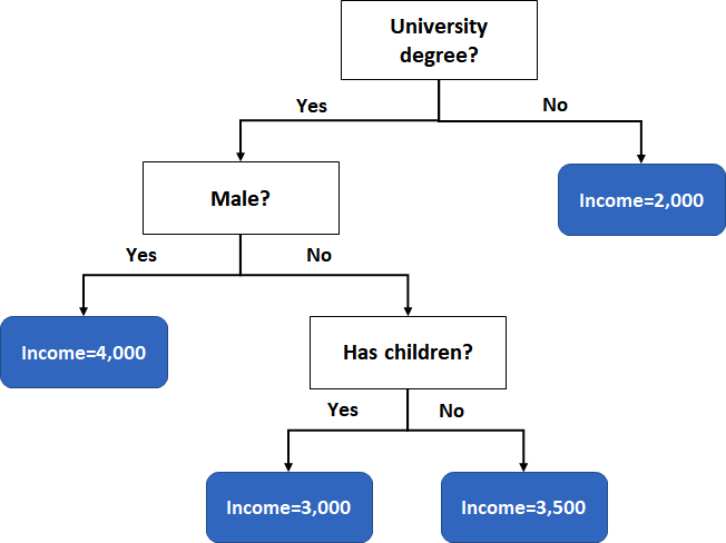
The second type of decision trees describes a regression model. For instance, take a look at the average income of a person based on different attributes.

Building a Decision Tree
When creating a decision tree, it is our ambition to increase the impurity of the data. That is looking for “good splits” that reduce the impurity and avoiding splits that only fit for few data points.
To measure impurity \(\small{ I\left(N\right) }\) of some node \(\small{ N }\), there are several common choices to take. Two often used impurity criteria are the Entropy \(\small{ I_E\left(N\right) }\) and the Gini Index \(\small{ I_G\left(N\right) }\).
Entropy:
\[I_E\left(N\right)=-\sum_{j=1}^{c}{p_j\log_2{(p_j)}}\]
Gini Index:
\[I_G\left(N\right)=1-\sum_{j=1}^{c}p_j^2\]
\(\small{ p_j=p(y_j|N) }\) denotes the proportion of data points that belongs to class \(\small{ c }\) for node \(\small{ N }\) . The Gini Index can reach a maximum of \(\small{ max{\ I}G\left(N\right)=0.5 }\) and with Entropy \(\small{ max{\ I}_E\left(N\right)=1 }\). Using the impurity criteria, we can now derive a new measure that indicates the goodness-of-split:
The Information Gain Criterion \(\small{ IG\left(N\right) }\) is the weighted mean decrease in impurity and is denoted as
\[IG\left(N\right)=I\left(N\right)-p{N1}\ast\ I\left(N_1\right)-p_{N2}\ast\ I\left(N_2\right)\]
To find the best split, a comparison of \(\small{ IG\left(N\right) }\) to all other possible splits is required.
Pseudo-Code for Building a Decision Tree
Input:
 S	//Set of data points

Algorithm:
 Start from root node with all the data
 Repeat:
   1.	For each variable find the best split
   2.	Compare best splits per variable across all variables
   3.	Select best overall split and optimal threshold
   4.	Split tree and create two branches
 Until: No further improvement is possible

Output:
 Decision Tree
Algorithms of decision trees tend to build their models very close to the training data and sometimes “learn it by heart”. As already mentioned, this will lead to bad predictions on new testing data. We call this overfitting. Therefore, it is vital to apply stopping criteria on the tree growing. The model applies “pre-pruning” if it does not fully grow the complete decision tree and it applies “post-pruning” it first grows fully the tree and then cut branches that do not add much information.

